Building a Neural Network from Scratch

When I followed Andrew Ng’s Neural Networks and Deep Learning course on Coursera, I found building a Neural Network from scratch extremely helpful to get a clear understanding of how these work. In this post, I share with you how I built a deep neural network from scratch to get a better understanding of its inner workings.

The model is a classifier that distinguishes cat images from non-cat images. I start by building a 2-layer Neural Network, then a deeper 4-layer Network to compare how they perform.

Our models are basic neural networks and their performances are obviously not optimal for many reasons. Their performances can however be further improved notably via hyperparameter tuning such as exploring different network structures, depths, using regularization etc …

Please note that more information regarding references and the dataset can be found at the bottom of this post.

import time
import numpy as np
import h5py
import matplotlib.pyplot as plt
import scipy

import imageio
import scipy.misc
from PIL import Image
from scipy import ndimage


%matplotlib inline
plt.rcParams['figure.figsize'] = (5.0, 4.0) 
plt.rcParams['image.interpolation'] = 'nearest'
plt.rcParams['image.cmap'] = 'gray'

The dataset

We have a training dataset of 209 images and their labels (cat/non-cat) and a test dataset of 50 images and their labels stored in h5py files. Each image is a 64x64 pixel image. Let’s load the datasets and store the data in numpy arrays.

train_dataset = h5py.File('train_catvnoncat.h5', "r")
train_x_orig = np.array(train_dataset["train_set_x"][:]) 
train_y_orig = np.array(train_dataset["train_set_y"][:]) 

test_dataset = h5py.File('test_catvnoncat.h5', "r")
test_x_orig = np.array(test_dataset["test_set_x"][:]) 
test_y_orig = np.array(test_dataset["test_set_y"][:])

classes = np.array(test_dataset["list_classes"][:]) 
    
train_y = train_y_orig.reshape((1, train_y_orig.shape[0]))
test_y = test_y_orig.reshape((1, test_y_orig.shape[0]))

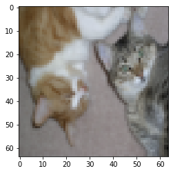
Let’s have a look at a few examples of our data set.

index = 162
plt.imshow(train_x_orig[index])
print ("y = " + str(train_y[0,index]) + ". This is a " + classes[train_y[0,index]].decode("utf-8") +  " picture.")

y = 1. This is a cat picture.

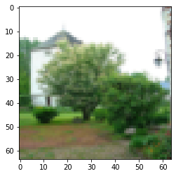
index = 55

plt.imshow(train_x_orig[index])
print ("y = " + str(train_y[0,index]) + ". This is a " + classes[train_y[0,index]].decode("utf-8") +  " picture.")

y = 0. This is a non-cat picture.

Now let’s have a look at our variables dimensions. Our training inputs train_x_orig.shape is (209, 64, 64, 3): it has 209 images, each of shape (64x64x3) where 64 is the height and width of the image in pixels and 3 the number of channels (RGB).

m_train = train_x_orig.shape[0]
num_px = train_x_orig.shape[1]
m_test = test_x_orig.shape[0]

print ("train_x_orig shape: " + str(train_x_orig.shape))
print ("train_y shape: " + str(train_y.shape))
print ("test_x_orig shape: " + str(test_x_orig.shape))
print ("test_y shape: " + str(test_y.shape)+ '\n')

print ("Number of training examples: " + str(m_train))
print ("Number of testing examples: " + str(m_test))
print ("Each image is of size: (" + str(num_px) + ", " + str(num_px) + ", 3)")

train_x_orig shape: (209, 64, 64, 3)
train_y shape: (1, 209)
test_x_orig shape: (50, 64, 64, 3)
test_y shape: (1, 50)

Number of training examples: 209
Number of testing examples: 50
Each image is of size: (64, 64, 3)

In the below we reshape our images into vectors to prepare them to be fed to the neural network. We reshape each (64, 64, 3) image into an image vector of shape (64 * 64 * 3, 1).

The resulting training set is a matrix with 64 * 64 * 3 rows and 209 (Number of training examples) columns, and the resulting test set is a matrix with 64 * 64 * 3 rows and 50 columns (Number of testing examples). The “-1” in reshape() flattens the remaining dimensions.

train_x_flatten = train_x_orig.reshape(train_x_orig.shape[0], -1).T   
test_x_flatten = test_x_orig.reshape(test_x_orig.shape[0], -1).T

print('flatttened training set shape: ' + str(train_x_flatten.shape))
print('flatttened testing set shape: ' + str(test_x_flatten.shape))

flatttened training set shape: (12288, 209)
flatttened testing set shape: (12288, 50)

We standardize our feature values so they are on a similar scale by dividing each pixel value by 255. The resulting feature values are all between 0 and 1

train_x = train_x_flatten/255.
test_x = test_x_flatten/255.

Implementing helper functions

For each of our models, we follow the below steps:

• define the model’s structure - number of layers, number of units in each layer and its activation function
• initialize the model’s weights and biases for each layer
• loop for a number of iterations where each iteration is a step of the Gradient Descent algorithm to minimize the loss function: 1. perform forward propagation to compute the activations at each layer 2. compute the cross-entropy cost 3. perform back propagation to compute gradients at each layer 4. update weights and biases
• predict the labels of the test set using the trained model

To implement each of the above steps, we will implement functions initialize_parameters(), linear_activation_forward(), compute_cost(), linear_activation_backward() and update_parameters().

Initialize parameters

In the initialize_parameters() function we randomly initialize our weights Wl to numbers between 0 and 0.01 and our bias b to zeros.

• We do not want our weights to be large, because these would lead to high activations, where the learning of the network will be too slow due to very small gradients.
• We do not want to initialize our weights to zeros because in this case our model will fail to break symmetry and won’t allow different units to learn independently of each other.
• It is ok to initialize our bias vectors to zeros.

Please note that our initialize_parameters() will also be used for our deeper network where initialization will be slightly different, as we will perform He initialization He et al., Delving Deep into Rectifiers.

def initialize_parameters(layer_dims):
    parameters = {}
    L = len(layer_dims)  
      
    if L <=3:
        W1 = np.random.randn(layer_dims[1], layer_dims[0])*0.01
        b1 = np.zeros((layer_dims[1], 1))
        W2 = np.random.randn(layer_dims[2], layer_dims[1])*0.01
        b2 = np.zeros((layer_dims[2], 1))
       
        parameters = {"W1": W1,"b1": b1,"W2": W2,"b2": b2}
        
    else:
        for l in range(1, L):
            parameters['W' + str(l)] = np.random.randn(layer_dims[l], layer_dims[l-1]) / np.sqrt(layer_dims[l-1])
            parameters['b' + str(l)] = np.zeros((layer_dims[l], 1))   
  
    return parameters    

Forward propagation

The linear_activation_forward() function defined below takes as inputs the activation from the previous layer A_prev, the weights W and bias b for the current layer and the activation function (either ReLU for the hidden layer or Sigmoid for the output layer in our case). It returns the activation A for the current layer, as well as a cache where the value of vector Z is stored to be used in the backward propagation.

For layer $ l $, the function computes

and

where g is ReLu: $ g(Z) = max(0, Z) $ for the hidden layer and sigmoid $ g(Z) = \frac{1}{1 + e^{-Z}} $ for the output layer.

def linear_activation_forward(A_prev, W, b, activation):
    Z = np.dot(W, A_prev) + b
    linear_cache = (A_prev, W, b)
    
    if activation == "sigmoid":
        A = 1/(1+np.exp(-Z))
    
    elif activation == "relu":
        A = np.maximum(0, Z)
    
    activation_cache = Z
    cache = (linear_cache, activation_cache)

    return A, cache

Compute cross-entropy cost

The compute_cost() function computes the cross-entropy cost $J$, using the following formula:

def compute_cost(AL, Y):
    m = Y.shape[1]

    cost = -(1./m) * (np.sum(Y*np.log(AL)) + np.sum((1-Y)*np.log(1-AL)))
    
    cost = np.squeeze(cost)      
    return cost

Backward propagation

The linear_activation_backward() function defined below takes as inputs the gradient of the activation dA, and the cache that was computed during the forward propagation, containing Z, weights W and bias b for the current layer and the activation function (either ReLU for the hidden layer or Sigmoid for the output layer in our case). It returns the activation gradient dA for the previous layer, as well as the gradients of the weignts dW and db.

If our current layer is $ l $, the function computes

def linear_activation_backward(dA, cache, activation):
   
    linear_cache, activation_cache = cache
    
    Z = activation_cache
    A_prev, W, b = linear_cache
    
    if activation == "relu":
        dZ = np.array(dA, copy = True)
        dZ[Z <= 0] = 0
                
    elif activation == "sigmoid":
        s = 1/(1+np.exp(-Z))
        dZ = dA * s * (1-s)
     
    m = A_prev.shape[1]
    dW = 1./m * np.dot(dZ,A_prev.T)
    db = 1./m * np.sum(dZ, axis = 1, keepdims = True)
    dA_prev = np.dot(W.T,dZ)
    
    return dA_prev, dW, db

Update parameters

Function update_parameters() will update the weights W and bias b of the model, using gradient descent:

where $\alpha$ is the learning rate.

def update_parameters(parameters, grads, learning_rate):
      
    L = len(parameters) // 2

    for l in range(L):
        parameters["W" + str(l+1)] = parameters["W" + str(l+1)] - learning_rate * grads["dW" + str(l+1)]
        parameters["b" + str(l+1)] = parameters["b" + str(l+1)] - learning_rate * grads["db" + str(l+1)]
        
    return parameters

Two layer model

Function two_layer_model() puts together the functions defined above: it calls initalize_parameters() to randomly initialize weights and bias for the two layers of the model. Then, it performs num_iterations gradient descent steps, where is each step, it:

• calls the linear_activation_forward() function to compute activation on layer 1 and 2
• calls the compute_cost() function to compute the cross-entropy cost with the current parameters
• calls the linear_activation_backward() function to compute gradients of the activation and parameters
• calls the update_parameters() function to update weights and bias using the computed gradients and the learning rate.

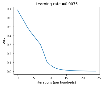
It keeps track of the cost at every 100 iterations of the gradient descent, and outputs a plot of the cost as a function of the number of iterations.

def two_layer_model(X, Y, layers_dims, learning_rate = 0.0075, num_iterations = 3000, print_cost=False):
     
    grads = {}
    costs = []                              
    m = X.shape[1]                           
    
    
    parameters = initialize_parameters(layers_dims)
    
    W1 = parameters["W1"]
    b1 = parameters["b1"]
    W2 = parameters["W2"]
    b2 = parameters["b2"]
    
 
    for i in range(0, num_iterations):

        A1, cache1 = linear_activation_forward(X, W1, b1, "relu")
        A2, cache2 = linear_activation_forward(A1, W2, b2, "sigmoid")

        cost = compute_cost(A2, Y)
        
        dA2 = - (np.divide(Y, A2) - np.divide(1 - Y, 1 - A2))
        

        dA1, dW2, db2 = linear_activation_backward(dA2, cache2, "sigmoid")
        dA0, dW1, db1 = linear_activation_backward(dA1, cache1, "relu")
        
        grads['dW1'] = dW1
        grads['db1'] = db1
        grads['dW2'] = dW2
        grads['db2'] = db2
        

        parameters = update_parameters(parameters, grads, learning_rate)

        W1 = parameters["W1"]
        b1 = parameters["b1"]
        W2 = parameters["W2"]
        b2 = parameters["b2"]
        
        if print_cost and i % 100 == 0:
            print("Cost after iteration {}: {}".format(i, np.squeeze(cost)))
        if i % 100 == 0:
            costs.append(cost)
       
    plt.plot(np.squeeze(costs))
    plt.ylabel('cost')
    plt.xlabel('iterations (per hundreds)')
    plt.title("Learning rate =" + str(learning_rate))
    plt.show()
    
    return parameters

L layer helper functions

L_model_forward() function will be used for our L layer Deep Neural Network. It simply loops through all the layers of the network and calls linear_activation_forward() on each layer. It records the cache containing Z values for all layer in a list, which it returns along with the computed activation for the last layer of the network.

def L_model_forward(X, parameters):

    caches = []
    A = X
    L = len(parameters) // 2                
    
    for l in range(1, L):
        A_prev = A 
        A, cache = linear_activation_forward(A_prev, parameters['W' + str(l)], parameters['b' + str(l)], activation = "relu")
        caches.append(cache)
    
    AL, cache = linear_activation_forward(A, parameters['W' + str(L)], parameters['b' + str(L)], activation = "sigmoid")
    caches.append(cache)
    
       
    return AL, caches

L_model_backward() function will be used for our L layer Deep Neural Network. It simply loops through all the layers of the network and calls linear_activation_backward() on each layer. It records and returns a dictionary containing the gradients computed at each later of the network.

def L_model_backward(AL, Y, caches):
   
    grads = {}
    L = len(caches) 
    m = AL.shape[1]
    Y = Y.reshape(AL.shape) 
    
    dAL = - (np.divide(Y, AL) - np.divide(1 - Y, 1 - AL))
    
    current_cache = caches[L-1]
    grads["dA" + str(L-1)], grads["dW" + str(L)], grads["db" + str(L)] = linear_activation_backward(dAL, current_cache, activation = "sigmoid")
    
    for l in reversed(range(L-1)):
        current_cache = caches[l]
        dA_prev_temp, dW_temp, db_temp = linear_activation_backward(grads["dA" + str(l + 1)], current_cache, activation = "relu")
        grads["dA" + str(l)] = dA_prev_temp
        grads["dW" + str(l + 1)] = dW_temp
        grads["db" + str(l + 1)] = db_temp

    return grads

Function L_layer_model() puts together the functions defined above to built a deep L-layer Neural Network: it calls initalize_parameters() to randomly initialize weights and bias for the L layers of the model. Then, it performs num_iterations gradient descent steps, where is each step, it:

• calls the L_model_forward() function to compute activations at layer L - the output layer
• calls the compute_cost() function to compute the cross-entropy cost with the current parameters
• calls the L_model_backward() function to compute gradients of the activation and parameters
• calls the update_parameters() function to update weights and bias using the computed gradients and the learning rate.

It keeps track of the cost at every 100 iterations of the gradient descent, and outputs a plot of the cost as a function of the number of iterations.

def L_layer_model(X, Y, layers_dims, learning_rate = 0.0075, num_iterations = 3000, print_cost=False):

    costs = []                       
    
    parameters = initialize_parameters(layers_dims)
    
    for i in range(0, num_iterations):

        AL, caches = L_model_forward(X, parameters)
        
   
        cost = compute_cost(AL, Y)
  
        grads = L_model_backward(AL, Y, caches)
 
        parameters = update_parameters(parameters, grads, learning_rate)
               
        if print_cost and i % 100 == 0:
            print ("Cost after iteration %i: %f" %(i, cost))
        if  i % 100 == 0:
            costs.append(cost)
            
    plt.plot(np.squeeze(costs))
    plt.ylabel('cost')
    plt.xlabel('iterations (per hundreds)')
    plt.title("Learning rate =" + str(learning_rate))
    plt.show()
    
    return parameters

Predict Function

Function predict() will use the parameters of the model we end up with after going through our gradient descent iterations, it takes X, a set of images, and a corresponding set of labels y as parameters and computes probabilities p of each input being a cat image based on the trained model’s parameters.

If p is greater than 0.5, the function predicts that the image is a cat image. If not, it predicts that the image is a non-cat image. It then compared its prediction to the actual image label, and computed an accuracy rate for the whole set.

def predict(X, y, parameters):
   
    m = X.shape[1]
    n = len(parameters) // 2 
    p = np.zeros((1,m))
    
    probas, caches = L_model_forward(X, parameters)
  
    for i in range(0, probas.shape[1]):
        if probas[0,i] > 0.5:
            p[0,i] = 1
        else:
            p[0,i] = 0
    
    print("Accuracy: "  + str((np.sum((p == y)/m))))
        
    return p

Building a 2 layer Neural Network

Let’s now build a 2 layer model and train it using our training set of images. The below constants define our model’s structure:

• The input layer X has n_x = 12,288 units corresponding to the number of features of each input image (64 x 64 x 3).
• We chose to give our hidden layer n_h = 7 units.
• Our output layer has one unit

n_x = 64*64*3
n_h = 7
n_y = 1
layers_dims = (n_x, n_h, n_y)

parameters = two_layer_model(train_x, train_y, layers_dims = (n_x, n_h, n_y), num_iterations = 2500, print_cost=False)

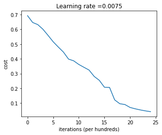
The 2-layer network has an accuracy of 72% on the test set. Let’s see if a deeper neural network is any more accurate.

print("On training set: ") 
predictions_train = predict(train_x, train_y, parameters)
print("On test set: ") 
predictions_test = predict(test_x, test_y, parameters)

On training set: 
Accuracy: 0.9999999999999998
On test set: 
Accuracy: 0.7299999999999999

Building a deeper, 4-layer Neural Network

Let’s now build a deeper model - let’s build a 4 layer model and train it using our training set of images. Our model will have 1 input layer, 3 hidden layers with 20, 7 and 5 units respectively and an output layer of 1 unit. layer_dim list below describes the structure of the network.

We will train the network on our training set, for 2500 iterations.

layers_dims = [12288, 20, 7, 5, 1]
parameters = L_layer_model(train_x, train_y, layers_dims, num_iterations = 2500, print_cost = False)

Our 4 layer model predicts the labels of our test set with 80% accuracy!! Which is a great improvement from the 2 layer model. These performances are not optimal and can be further improved via hyperparameter tuning such as exploring different network structures, depths, using regularization etc …

print("On training set: ") 
pred_train = predict(train_x, train_y, parameters)
print("On test set: ") 
pred_test = predict(test_x, test_y, parameters)

On training set: 
Accuracy: 0.9999999999999998
On test set: 
Accuracy: 0.8

Testing the model on a new image

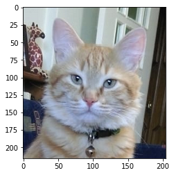
Let’s see how the model classifies an image of Loulou :heart:

fname = "loulou_face.png" 
label_y = [1] 

image = np.array(imageio.imread(fname, as_gray=False, pilmode="RGB"))

plt.imshow(image)

<matplotlib.image.AxesImage at 0x7fcfc3d00fa0>

my_image = np.array(Image.fromarray(image).resize(size=(num_px,num_px)))
my_image = my_image.reshape(1, -1).T
my_image = my_image/255.

my_predicted_image = predict(my_image, label_y, parameters)

print ("y = " + str(np.squeeze(my_predicted_image)) + ", your L-layer model predicts a \"" + classes[int(np.squeeze(my_predicted_image)),].decode("utf-8") +  "\" picture.")

Accuracy: 1.0
y = 1.0, your L-layer model predicts a "cat" picture.

Note

Please note that this post is inspired by the programming assignments of the Neural Networks and Deep Learning course on Coursera. It uses the same dataset.