Michèle Srour Data Scientist
ATP linear regression

In this notebook we are going to explore data from the men’s professional tennis league, which is called the ATP (Association of Tennis Professionals). We are going to familiarize ourselves with the data, analyse it, and build a model that predicts the outcome for a tennis player based on their playing habits.
The data on-hand is about the top 1500 ranked players in the ATP over the span of 2009 to 2017. The statistics recorded for each player in each year include service game (offensive) statistics, return game (defensive) statistics and outcomes. The different fields in the data set are described in the appendix at the end of this notebook.
Importing librairies
import pandas as pd
import matplotlib.pyplot as plt
import seaborn as sns

from scipy.stats import pearsonr
from sklearn.model_selection import train_test_split
from sklearn.linear_model import LinearRegression
Importing the data from ‘tennis_stats.csv’ in a Pandas dataframe and displaying the first few lines of the data
df = pd.read_csv('tennis_stats.csv')
df.head()
| Player | Year | FirstServe | FirstServePointsWon | FirstServeReturnPointsWon | SecondServePointsWon | SecondServeReturnPointsWon | Aces | BreakPointsConverted | BreakPointsFaced | ... | ReturnGamesWon | ReturnPointsWon | ServiceGamesPlayed | ServiceGamesWon | TotalPointsWon | TotalServicePointsWon | Wins | Losses | Winnings | Ranking | |
|---|---|---|---|---|---|---|---|---|---|---|---|---|---|---|---|---|---|---|---|---|---|
| 0 | Pedro Sousa | 2016 | 0.88 | 0.50 | 0.38 | 0.50 | 0.39 | 0 | 0.14 | 7 | ... | 0.11 | 0.38 | 8 | 0.50 | 0.43 | 0.50 | 1 | 2 | 39820 | 119 |
| 1 | Roman Safiullin | 2017 | 0.84 | 0.62 | 0.26 | 0.33 | 0.07 | 7 | 0.00 | 7 | ... | 0.00 | 0.20 | 9 | 0.67 | 0.41 | 0.57 | 0 | 1 | 17334 | 381 |
| 2 | Pedro Sousa | 2017 | 0.83 | 0.60 | 0.28 | 0.53 | 0.44 | 2 | 0.38 | 10 | ... | 0.16 | 0.34 | 17 | 0.65 | 0.45 | 0.59 | 4 | 1 | 109827 | 119 |
| 3 | Rogerio Dutra Silva | 2010 | 0.83 | 0.64 | 0.34 | 0.59 | 0.33 | 2 | 0.33 | 5 | ... | 0.14 | 0.34 | 15 | 0.80 | 0.49 | 0.63 | 0 | 0 | 9761 | 125 |
| 4 | Daniel Gimeno-Traver | 2017 | 0.81 | 0.54 | 0.00 | 0.33 | 0.33 | 1 | 0.00 | 2 | ... | 0.00 | 0.20 | 2 | 0.50 | 0.35 | 0.50 | 0 | 1 | 32879 | 272 |
5 rows × 24 columns
Analysing the relationship between different features of the data set and the amount of Winnings
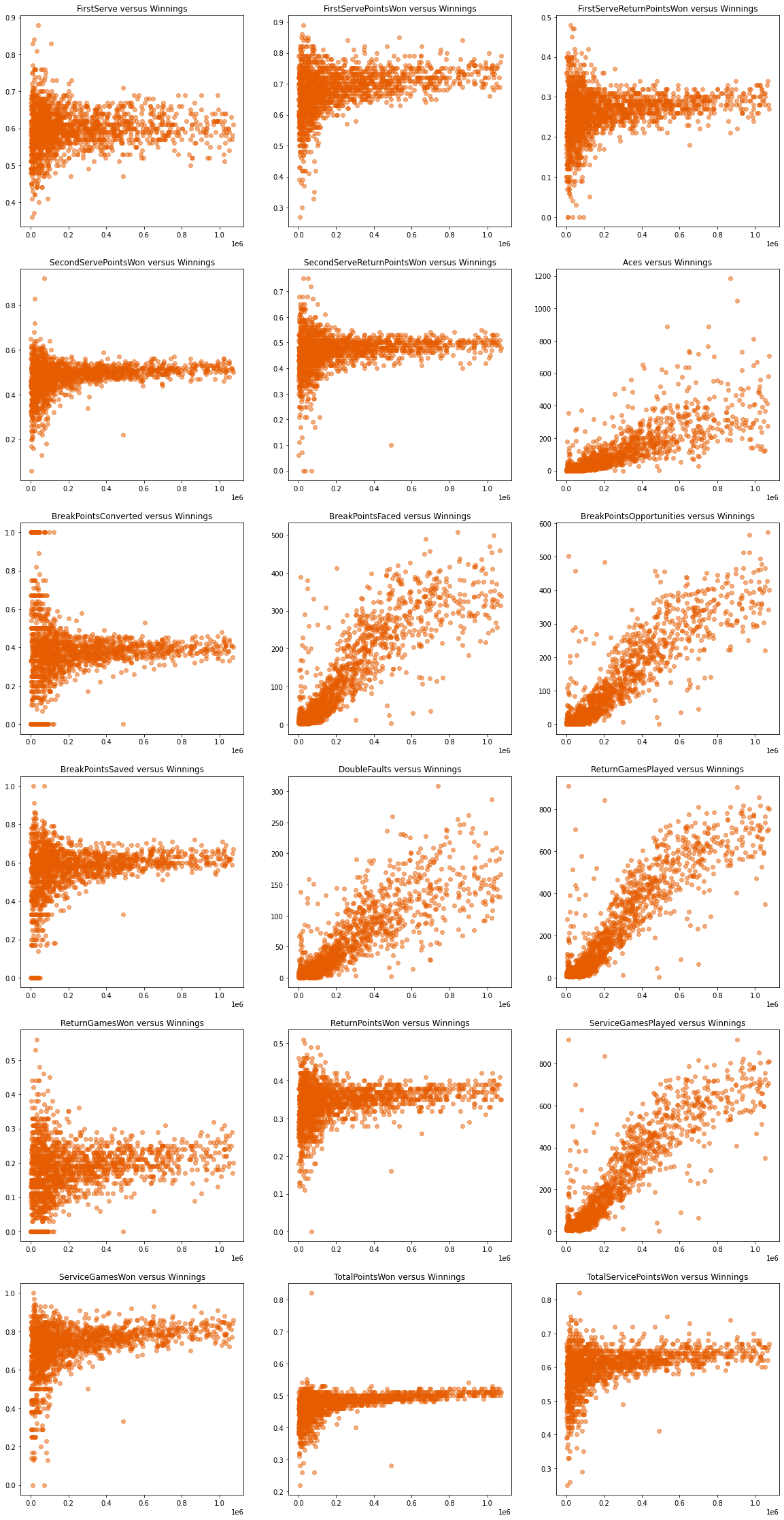
Plotting different features against Winnings to identify patterns. There appears to be a strong positive linear relationship between BreakPointsFaced, BreakPointsOpportunities, ReturnGamesPlayed, ServiceGamesPlayed and Winningss.
plt.figure(figsize = (20, 40))

features = ['FirstServe', 'FirstServePointsWon', 'FirstServeReturnPointsWon', 'SecondServePointsWon',
       'SecondServeReturnPointsWon', 'Aces', 'BreakPointsConverted','BreakPointsFaced', 'BreakPointsOpportunities', 'BreakPointsSaved',
       'DoubleFaults', 'ReturnGamesPlayed', 'ReturnGamesWon','ReturnPointsWon', 'ServiceGamesPlayed', 'ServiceGamesWon',
       'TotalPointsWon', 'TotalServicePointsWon']

for index in range(len(features)):
    ax = plt.subplot(6, 3, index + 1)
    title = features[index] + " versus Winnings"
    ax.title.set_text(title)
    plt.scatter(df["Winnings"], df[features[index]], alpha = 0.5, color = "#e65c00")

plt.show()
Calculating the Pearson Correlation between Winnings and all other features to identify those that have a strong linear relationship with Winnings.
features = ['FirstServe', 'FirstServePointsWon', 'FirstServeReturnPointsWon', 'SecondServePointsWon',
       'SecondServeReturnPointsWon', 'Aces', 'BreakPointsConverted','BreakPointsFaced', 'BreakPointsOpportunities', 'BreakPointsSaved',
       'DoubleFaults', 'ReturnGamesPlayed', 'ReturnGamesWon','ReturnPointsWon', 'ServiceGamesPlayed', 'ServiceGamesWon',
       'TotalPointsWon', 'TotalServicePointsWon']

for index in range(len(features)):
    corr, p = pearsonr(df["Winnings"], df[features[index]])
    if corr > 0.40 or corr< -0.40:
        print(features[index],": " , round(corr , 4))
Aces :  0.7984
BreakPointsFaced :  0.876
BreakPointsOpportunities :  0.9004
DoubleFaults :  0.8547
ReturnGamesPlayed :  0.9126
ServiceGamesPlayed :  0.913
TotalPointsWon :  0.4611
TotalServicePointsWon :  0.4077
Building a single feature linear regression model to predict Winnings
Based on the above, we’ve identified a strong linear relationship between Winnings and each of the following features: BreakPointsOpportunities, ReturnGamesPlayed and ServiceGamesPlayed.
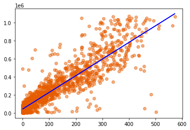
We are going to build and train a single feature linear regression model using the BreakPointsOpportunities feature to predict Winnings and use sklearn‘s LinearRegression .score() method that returns the coefficient of determination R² of the prediction to assess the model’s accuracy.
x = df[['BreakPointsOpportunities']]
y = df['Winnings']

x_train, x_test, y_train, y_test = train_test_split(x, y, train_size = 0.8, test_size = 0.2, random_state=6)

singlefeature_lr = LinearRegression()
singlefeature_lr.fit(x_train, y_train)

print("The coefficient of determination R² of the single feature prediction:")
print(" - on the training data: ", singlefeature_lr.score(x_train, y_train))
print(" - on the test data: ", singlefeature_lr.score(x_test, y_test))
The coefficient of determination R² of the single feature prediction:
 - on the training data:  0.8111412774695739
 - on the test data:  0.8081205523550063
y_predict = singlefeature_lr.predict(x)

plt.scatter(df['BreakPointsOpportunities'], df['Winnings'], alpha = 0.5, color = '#e65c00')
plt.plot(x, y_predict, color = 'Blue')
plt.show()
Building a two-feature linear regression model to predict Winnings
Based on the above, we’ve identified a strong linear relationship between Winnings and each of the following features:
BreakPointsOpportunities
ReturnGamesPlayed
ServiceGamesPlayed
We are going to build and train a linear regression model using the ReturnGamesPlayed and the ServiceGamesPlayed features to predict Winnings.
x = df[['BreakPointsOpportunities', 'ServiceGamesPlayed']]
y = df[['Winnings']]

x_train, x_test, y_train, y_test = train_test_split(x, y, train_size = 0.8, test_size = 0.2, random_state=6)

two_features_lr = LinearRegression()
two_features_lr.fit(x_train, y_train)

print("The coefficient of determination R² of the two-feature prediction:")
print(" - on the training data: ", two_features_lr.score(x_train, y_train))
print(" - on the test data: ", two_features_lr.score(x_test, y_test))
The coefficient of determination R² of the two-feature prediction:
 - on the training data:  0.8356666278203743
 - on the test data:  0.8303528220567031
Building a multiple-feature linear regression model to predict Winnings
Based on the above, we’ve identified a strong linear relationship (corr > 40) between Winnings and each of the following features:
Aces : corr = 0.7984
BreakPointsFaced : corr = 0.876
BreakPointsOpportunities : corr = 0.9004
DoubleFaults : corr = 0.8547
ReturnGamesPlayed : corr = 0.9126
ServiceGamesPlayed : corr = 0.913
TotalPointsWon : corr = 0.4611
TotalServicePointsWon : corr = 0.4077
x = df[['Aces', 'BreakPointsFaced', 'BreakPointsOpportunities', 'DoubleFaults', 'ReturnGamesPlayed', 'ServiceGamesPlayed', 'TotalPointsWon', 'TotalServicePointsWon']]
y = df[['Winnings']]

x_train, x_test, y_train, y_test = train_test_split(x, y, train_size = 0.8, test_size = 0.2, random_state=6)

mult_features_lr = LinearRegression()
mult_features_lr.fit(x_train, y_train)


print("The coefficient of determination R² of the multi-feature prediction:")
print(" - on the training data: ", mult_features_lr.score(x_train, y_train))
print(" - on the test data: ", mult_features_lr.score(x_test, y_test))
The coefficient of determination R² of the multi-feature prediction:
 - on the training data:  0.8442889601539872
 - on the test data:  0.8290095725876743
Conclusion
The above shows that we managed to improve the accuracy of the single feature model on the test dataset by adding a second feature. However, using 8 features in our linear regression model cause the accuracy on the test dataset to decrease due to overfitting the model to the training data.
Appendix
The different fields in the data set are described below:
Player: name of the tennis player
Year: year data was recorded
Service Game Columns (Offensive)
Aces: number of serves by the player where the receiver does not touch the ball
DoubleFaults: number of times player missed both first and second serve attempts
FirstServe: % of first-serve attempts made
FirstServePointsWon: % of first-serve attempt points won by the player
SecondServePointsWon: % of second-serve attempt points won by the player
BreakPointsFaced: number of times where the receiver could have won service game of the player
BreakPointsSaved: % of the time the player was able to stop the receiver from winning service game when they had the chance
ServiceGamesPlayed: total number of games where the player served
ServiceGamesWon: total number of games where the player served and won
TotalServicePointsWon: % of points in games where the player served that they won
Return Game Columns (Defensive)
FirstServeReturnPointsWon: % of opponents first-serve points the player was able to win
SecondServeReturnPointsWon: % of opponents second-serve points the player was able to win
BreakPointsOpportunities: number of times where the player could have won the service game of the opponent
BreakPointsConverted: % of the time the player was able to win their opponent’s service game when they had the chance
ReturnGamesPlayed: total number of games where the player’s opponent served
ReturnGamesWon: total number of games where the player’s opponent served and the player won
ReturnPointsWon: total number of points where the player’s opponent served and the player won
TotalPointsWon: % of points won by the player
Outcomes
Written on February 3rd , 2021Wins: number of matches won in a year
Losses: number of matches lost in a year
Winnings: total winnings in USD($) in a year
Ranking: ranking at the end of year